MLSS 2020 Notes: Causality

I try to consolidate my MLSS 2020 notes in small blog posts and hope you might also find them interesting. I don’t try to cover the complete lectures but rather pick some pieces that I find important when working or doing research in ML. I anticipate this series of blog posts will range from extremely superficial to excessively detailed for some readers.

I will start with Bernhard Schölkopf’s lecture on Causality (the second part by Stefan Bauer can be found here) and draw some connections to Moritz Hardt’s presentations (1 and 2) on fairness. I also recommend taking a look at Bernhard’s very accessible monograph.

Independence of Events and Random Variables

Before we start, we define some basic notions. The first one is the statistical independence of events. Let’s consider the events “rainy day” $R$ and “choosing Cini Minis as breakfast cereal” $C$ together with their respective probabilities $Pr(\cdot)$. If rain does not influence your cereal choice, and you can’t change the weather by eating Cini Minis, we say the events are independent, and the following equality holds: $$ Pr(R \cap C) = Pr(R) \cdot Pr(C). $$ Similarly, we can define the independence of continuous random variables $X$ and $Y$. We write $$ X \mathrel{\unicode{x2AEB}} Y $$ for independent variables if for their probability density functions $f_X(x)$ and $f_Y(y)$ it holds that $$ f_{X,Y}(x,y) = f_X(x)f_Y(y) $$ for all $x$ and $y$.

For the next concept, we introduce a third random variable $Z$ on which we can condition $X$ and $Y$. If $X$ and $Y$ and conditionally independent given $Z$, we write $$ (X \mathrel{\unicode{x2AEB}} Y) | Z, $$ and for the joint probability density conditioned on $Z$, it holds that $f_{XY|Z}(x,y|z)=f_X(x|z)f_Y(y|z)$ for all $x$,$y$, and $z$ such that $f_Z(z)>0$. This simply translates to the fact that

if I know $Z$, knowing $X$ does not tell me anything additional about $Y$.

Why is this relevant for causality? The notion of whether or not two random variables are dependent or independent is essential to understand the underlying phenomena that govern this relationship. For example, if we consider the classic example of observing increased stork activity ($X$) and increased birth rate ($Y$), $X$ and $Y$ can depend on each other in two ways:

1. $X \rightarrow Y$: storks bring babies, or
2. $Y \rightarrow X$: babies attract storks.

If we believe that both causal relationships are nonsensical, there must be a third factor that influences both observations simultaneously, $X$ and $Y$ have a common cause $Z$:

      3. $X \leftarrow Z \rightarrow Y$.

The fact that there is an underlying mechanism ($Z$) that explains the observed dependence is also known as the common cause principle [1]. Importantly, we cannot determine which of the three relationships is the “truth” given observational data alone.

Structural Causal Model

One approach to model such relationships/dependencies is structural causal models (SCM) [2], realized as directed acyclic graph (DAG) as shown below. Directed because we have arrows in one direction, rather than “simple” edges. Acyclic because there are no self-references. Vertices are observables (see further down for an analysis of the meaning of vertices with respect to fairness in AI), and arrows represent direct causation.

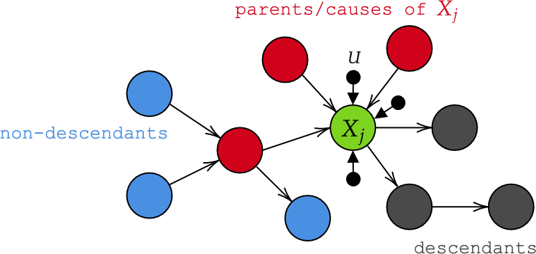
In the above graph, we say that an observable $X$, modeled as a random variable, is a function¹ of its parents $PA$ and exogenic or noise variables $U$: $$ X_j = f_j(PA_j, U_j), \qquad (j=1, \dots, n). $$

Importantly, all noise variables $U$ are stochastic and jointly independent, which leads to the insight that the functional viewpoint $f_j(PA_j, U_j)$ can represent the general conditional distribution $p(X_j|PA_j)$. If the $U$s were not independent, there has to be another mechanism (which we called $Z$ in the stork example) that causes their dependence, and hence we’d have to add it in the diagram. But since this is not the case, the graph contains all potential factors, and we call it causally sufficient.

The functional representation of a node can expressed purely by the noise factors by recursively substituting the parent equations: $$ X_j = f_j(PA_j, U_j) = f_j(f_k(PA_k, U_k), U_j) = f_j(f_k(f_l(PA_l, U_j), U_k), U_j) = \dots = g_j(U_1, \dots, U_n) $$ Each $X_j$ is therefore a random variable and we get a joint distribution of $p(X_1, \dots, X_n)$ which we call the observational distribution.

Disentangled Factorization & Graphical Causal Inference

If a structural causal model (e.g., a graph $G$ as shown in Figure 1) exists, there exists a factorization of the observational distribution: $$ p(X_1, \dots, X_n) = \prod_ip(X_i, PA_i). $$ We call each $p(X_i, PA_i)$ a causal conditional or causal Markov kernel. Note that only conditionals that are exclusively conditioned on their parents are causal; they are statistically independent of non-descendants given the parents (this is the local causal Markov condition). We call this factorization disentangled/causal if 1. knowing a mechanism $p(X_i,PA_i)$ does not yield any information about another mechanism $p(X_j,PA_j)$ for $i \neq j$, and 2. changing one $p(X_i,PA_i)$ does not change $p(X_j,PA_j)$ for $i \neq j$.

Changing $X_j$, for example by setting it to a constant $X_j=const$, is also called intervention. Interventions are key operators in Pearl’s do-calculus, which I will not address here, but this blog post should help you understand the concept.

Graphical Causal Inference They key question is now: How can we recover the graph $G$ of an SCM from the observational distribution $p$ (a.k.a the data)? The answer sounds quite simple: We perform conditional independence testing by tracking how the noise information “spreads through the data”. To make a statement about the existence of a causal graph $G$ when we only see data, we have to assume that seeing data is enough to actually make a statement about $G$. This sounds tautological but is called faithfulness and can be formalized by writing

$$ (X \mathrel{\unicode{x2AEB}} Y | Z)_p \Rightarrow (X \mathrel{\unicode{x2AEB}} Y | Z)_G. $$ This means that from observed conditional independence, we can deduce the causal relationship of these variables. This, however, is hard to justify for finite data, and we need to make assumptions on the function classes $f_{\bullet}$ (see chapter 6 of Causality for Machine Learning for details).

That’s all I wanted to say about this topic. As I said, it is by no means exhaustive, but hopefully provides the lingo that helps to understand some of the basic concepts of causality.

Parallel to Fairness in AI: Ontological instability of causal vertices/observables

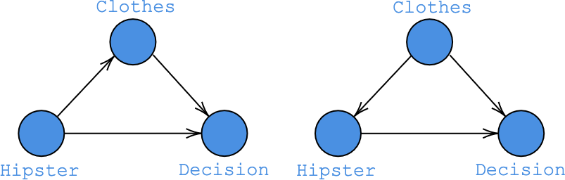
Moritz Hardt argued that we have to ask the fundamental question of what a node in a causal graph actually references. What is the ontological entity? He motivated this line of thought by considering the situation in which the job application of a person dressed like a hipster was rejected. There are now two positions we can take:

1. He was rejected because he is a hipster (being a hipster caused the rejection), and
2. He was rejected because he did not meet the dress code (his clothing caused the rejection).

In the first position, there is a mediator that conveyed that this person is a hipster (e.g., his clothes), which influenced the decision (left graph in Fig. 2). The second view stresses that being assigned the “hipster” label can be influenced by confounders such as clothing (right graph in Fig. 2).

The problem that clothing can be seen as either a mediator or a confounder, depending on the ontology that fits your world view best, is pointed out by Judea Pearl himself:

As you surely know by now, mistaking a mediator for a confounder is one of the deadliest sins in causal inference and may lead to the most outrageous error. The latter invites adjustment; the former forbids it. [4]

So the bigger question is: why can “hipster” even be a node in the first place? What does it reference, and what are its “settings”? In a more serious, but analogous situation (“she was rejected because of her religion”) we can take the same two views: Education acts as mediator for religion, and both influence the decision, or education is a confounder that determines religion (see Fairness in Decision-Making - The Causal Explanation Formula). According to Hardt, these competing models are manifestations of the suppressed question of what the “religion” node references in the first place. A similar problem arises from putting “race” in a causal model: What is race?

References

1. H. Reichenbach. 1956. The direction of time. University of California Press, Berkeley, CA.
2. J. Pearl. 2009. Causality: Models, Reasoning, and Inference. Cambridge University Press, New York, NY.
3. L. Lauritzen. 2009. Graphical models. Oxford University Press, New York, NY.
4. J. Pearl, and D. Mackenzie. The book of why: the new science of cause and effect. Basic Books, 2018.

1. Note, that $f$ does not refer to the probability density function as introduced in the beginning. It can be any function.