At last week’s ICDM, I presented our paper in which we derive a kernel for time series that uses notions of optimal transport (OT) theory. In this blog post, I am going to summarize our work by pointing out some caveats when naïvely constructing $\mathcal{R}$-convolution kernels for time series (TS), by introducing the Swiss Kantorovich problem 🇨🇭, and by describing our OT based TS kernel and its classification results on the UCR Time Series Classification Archive.
Caveats when constructing $\mathcal{R}$-convolution kernels for time series Link to heading
The $\mathcal{R}$-convolution framework [Haussler, 1999] is a popular way to construct kernels for structured data (e.g. text or graphs). It iteratively employs a base kernel $k_{\text{base}}(\cdot, \cdot)$ on the substructures of two objects $A$ and $B$ to compute the overall kernel:
$$ k_{\mathcal{R}}(A,B) = \sum_{a \in \text{sub}(A)}\sum_{b \in \text{sub}(B)} k_{\text{base}}(a,b) $$
The fact that the sum of two kernels results in a kernel (i.e. the kernel matrix is positive semi-definite (PSD)) makes this approach very powerful, as we can use it in kernel-based methods such as SVMs (e.g. for classification). So, to construct a kernel for time series classification (TSC), we only need to find some meaningful substructures of time series. Thankfully, the majority of current TSC methods do exactly this: They choose the $w$-length subsequences of a given time series as its representation to learn a classifier (or solve other ML related tasks). However, if we choose $k_{\text{base}}$ to be the linear kernel, $k_{\text{base}}(a,b)=a^{\top}b=\langle a,b\rangle$, $k_{\mathcal{R}}$ basically degenerates to the comparison of the means:
$$ k_{\mathcal{R}}(T,T’) = \sum_{s \in \mathcal{S}}\sum_{s’ \in \mathcal{S’}}k_{\text{base}}(s,s’) $$ $$ = \sum_{s \in \mathcal{S}}s^{\top}\sum_{s’ \in \mathcal{S’}}s’ \approx \bar{T}^\top \bar{T’}, $$
where $T$ and $T’$ are two time series and $\mathcal{S}$ and $\mathcal{S’}$ the sets of their subsequences of length $w$. The approximation comes from the fact that in the respective sums over all subsequence feature vectors, almost all of the observations of length $w$, except for the leading $w −1$ as well as the trailing $w−1$ observations, will appear at all dimensions of the vectors. This exacerbation is particularly problematic for TS as they are typically $z$-normalized. This leads to a kernel that effectively only “compares” zeros. Additionally, the $\mathcal{R}$-convolution framework for TS might not be ideal, as all subsequences from one TS are compared to all subsequences of a second TS. This makes the kernel less robust and prone to noise. Furthermore, we ignore the distribution of subsequences which might be of interest for periodic time series.
Our method tackles exactly these issues by using the Wasserstein metric, a distance measure for distributions, rooted in optimal transport theory. In the following I will give an intuitive explanation on how the optimal transport problem can be phrased and how the Wasserstein ($W_1$) distance is defined.
The Swiss Kantorovich Problem Link to heading
Before we start, I would like to point out that this description is largely motivated by Marco Cuturi’s Primer on Optimal Transport. Another great resource for the topic is the book “Computational Optimal Transport” by Gabriel Peyré and Marco Cuturi.
During World War II, Leonid Kantorovich, a soviet mathematician and economist, was concerned with moving soldiers from their base to the frontline, efficiently. It was know how many soldiers are in the bases and how many are needed at different locations at the front. Furthermore, we know the distances from each base to each battlefield. Here, we take a more “neutral” view on the same problem which I coin the “Swiss Kantorovich Problem”, depicted in Figure 1.
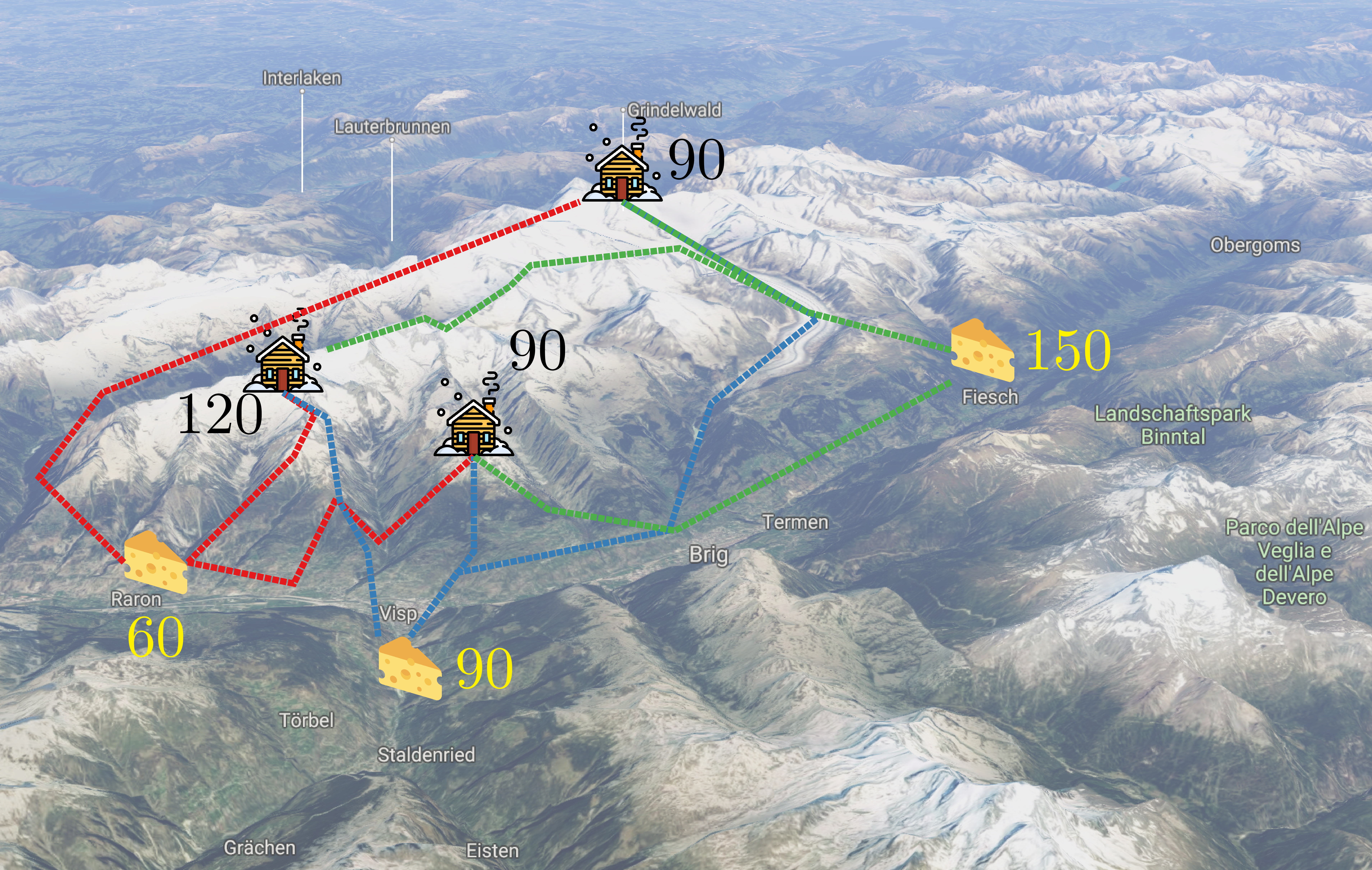
Imagine, you’re in the Swiss Alps and faced with the following problem: There are three cheese factories, they produce 60, 90, and 150 wheels of cheese, individually. At the same time, there are three ski huts which ran out of cheese and need 120, 90, and 90 wheels, individually. Unfortunately, there are only a limited number of paths connecting the factories and huts (dashed lines) and you want to distribute all cheese in a way that satisfies the needs of the huts and minimizes your effort (cheese wheels can be heavy).
Let us formalize this a little bit: The distances between huts and factories can be expressed in a matrix (Table 1) which we term ground distance matrix $D$. In our example, the entries could be the lengths of the individual connecting paths. To deliver cheese wheels, you must walk these paths and pull the cheese on a wagon. The effort of transporting $P$ cheese wheels from factory $i$ to hut $j$ can be expressed as $P_{i,j}D_{i,j}$. This brings us to the concept of the transport plan, a matrix $P$ (Table 2) of the same dimensions as $D$, which we’d like to fill in way that minimizes our effort or cost $C(P)$:
$$ C(P)=\sum_{i}\sum_j D_{i,j} P_{i,j}=\left\langle D, P \right\rangle_{\mathrm{F}} \text{ ,} $$
where $\left\langle D, P \right\rangle_{\mathrm{F}}$ is the Frobenius product.
| Hut a | Hut b | Hut c | |
| Factory 1 | $D_{1,a}$ | $D_{1,b}$ | $D_{1,c}$ |
| Factory 2 | $D_{2,a}$ | $D_{2,b}$ | $D_{2,c}$ |
| Factory 3 | $D_{3,a}$ | $D_{3,b}$ | $D_{3,c}$ |
| $m_a$ (120) | $m_b$ (90) | $m_c$ (90) | |
| $m_1$ (60) | $P_{1,a}$ | $P_{1,b}$ | $P_{1,c}$ |
| $m_2$ (90) | $P_{2,a}$ | $P_{2,b}$ | $P_{2,c}$ |
| $m_3$ (150) | $P_{3,a}$ | $P_{3,b}$ | $P_{3,c}$ |
In the search of $P$, we have to constrain ourselves to solutions that fulfill the requirement to get rid of all cheese and making all huts happy. Formally, these constraints can be expressed as:
$$ \sum_{j \in {a,b,c}}P_{i,j} = m_i \text{, } \forall{}i \in {1,2,3} \text{ and } \sum_{i \in {1,2,3}}P_{i,j} = m_j \text{, } \forall{}j \in {a, b, c} \text{ .} $$
The Frobenius product of $D$ and transportation plan $P$ that minimizes $C(P)$ is called $\text{1}^{st}$ Wasserstein distance:
$$ W_1\left(A, B\right) = \min_{P \in \Gamma\left(A, B\right)} \left\langle D, P \right\rangle_{\mathrm{F}}\text{ ,} $$
where $\Gamma\left(A, B\right)$ is the set of all valid (with respect to the constraints) transportation plans of $A$ and $B$. (Feel free to look at the paper to find out where the $1$ comes from)
A Wasserstein subsequence kernel for time series Link to heading
We already established that subsequences are a commonly used representation of time series. For now, we set the role of marginals aside and define all $m_i$ and $m_j$ to be equal to 1. We also replace huts by $\mathcal{S}$, i.e. the set of all $w$-length subsequences of time series $T$, and cheese factories by $\mathcal{S’}$, the subsequences of all length $w$ subsequences from time series $T’$. Furthermore, the ground distance matrix $D$ is defined as the pairwise euclidean distance of the subsequences in $\mathcal{S}$ and $\mathcal{S’}$. We can now directly use the distance definition from above to define a Wasserstein distance $W$ for time series:
$$ W(T, T’) = W_1(\mathcal{S}, \mathcal{S’}) \text{ .} $$
Given a time series data set with $n$ time series $\mathcal{T}=\{T_0, \dots, T_{n-1}\}$ , the Wasserstein distance matrix $\mathcal{W} \in \mathbb{R}^{n \times n}$ is defined as
$$ \mathcal{W}_{i,j} = W(T_i, T_j) \text{ .} $$
Our kernel (WTK) can eventually be constructed as a laplacian kernel:
$$ \text{WTK}\left(T_i, T_j\right) = \exp\left(-\lambda \mathcal{W}_{i,j}\right) \text{ .} $$
Note: We observe empirically that in some cases this does not lead to a positive definite kernel. We hence employ a Kreĭn SVM for our classification experiments which is capable of handling positive definite and indefinite kernel matrices.
A visual summary of WTK Link to heading
Figure 2 illustrates the components of our method for two time series and a subsequence length of $w=5$. It also showcases how the method intrinsically works for time series of varying lengths. Yellow cells indicate high values. For $D$, this means high euclidean distance between two subsequences. In $P$ each cell represents how much of the mass of a subsequence is distributed to other subsequences. The marginals of $P$ are all 1. Panel c) visualizes the alignment or matching that can be inferred from the transport plan. Similarly shaped subsequences, close in euclidean distance, are matched. Note that one subsequence can be mapped to multiple other subsequences as long as the rows and columns sum up to 1.
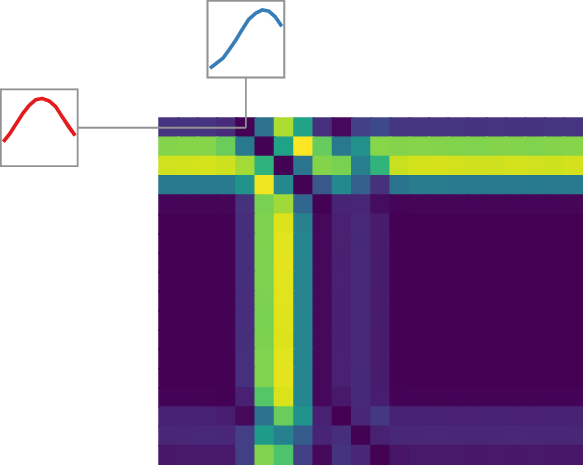 a) Ground distance matrix $D$
|
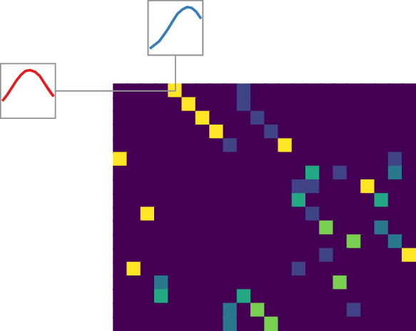 b) Optimal transport plan $P$
|
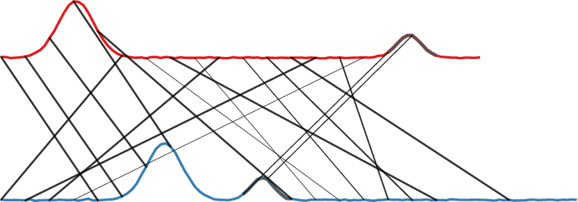 c) Subsequence matching following $P$
|
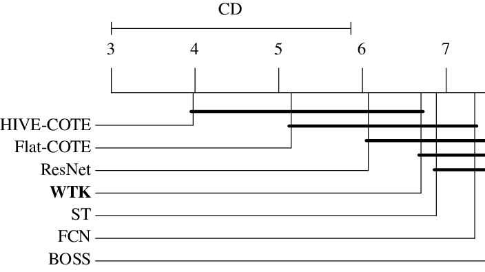
Classification Experiments Link to heading
We applied our method to 85 TSC data sets from the UCR Time Series Classification Archive. Each data set contains time series of equal length with a predefined train and test split. As noted above, we employed a Kreĭn SVM for classification and tuned hyperparameters in 5-fold cross-validation. The subsequence length $w$ was a tunable parameter consisting of 10%, 30%, and 50% of the time series length of respective data set. Figure 3 shows the interesting part of a critical difference plot in which we compare our method with all state-of-the-art TSC methods. Both COTE methods are ensemble methods that combine over 30 different TSC methods. The complete plot can be found in the paper.